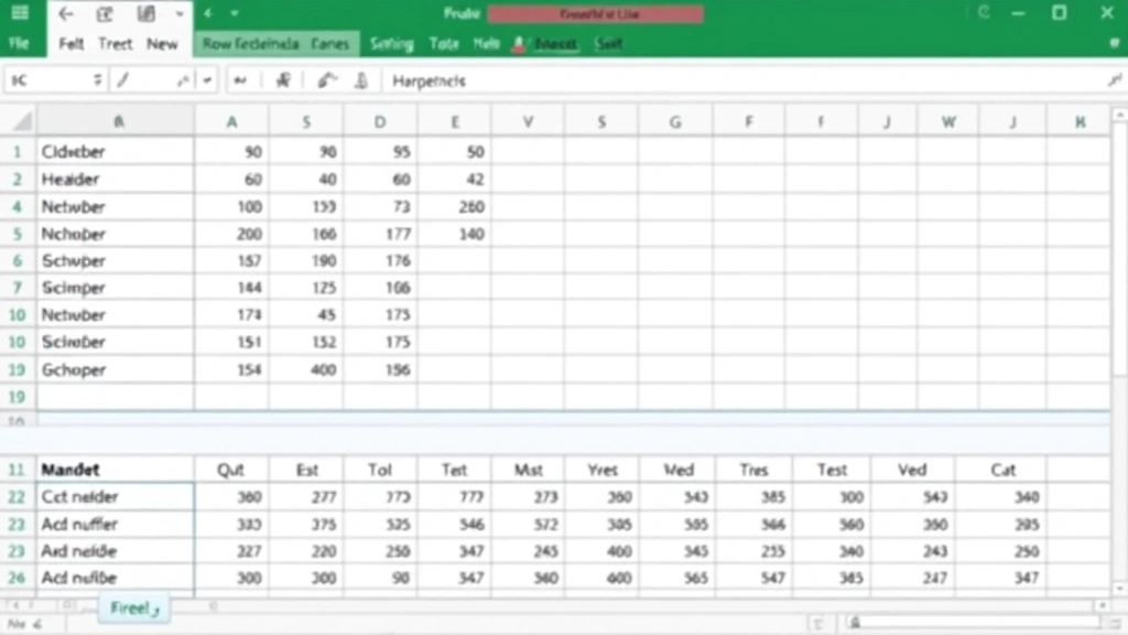
How to Freeze Cells in Excel: Step-by-Step Guide

If you’ve ever scrolled through a massive Excel spreadsheet and lost track of your column headers or row labels, you know the frustration. One moment you’re comparing data in row 50, and the next you’ve forgotten what each column represents. That’s where freezing cells comes in—a surprisingly simple yet powerful feature that keeps your reference points visible no matter how far you scroll.

Freezing cells in Excel is like pinning important information to your screen. Whether you’re managing a budget, tracking inventory, or analyzing sales data, this technique transforms how you work with large datasets. The best part? It takes just a few clicks, and once you understand the mechanics, you’ll wonder how you ever worked without it.

Let’s dive into everything you need to know about freezing cells, from the basics to advanced techniques that’ll make your spreadsheet navigation smoother than ever.

What Does Freezing Cells Mean?

Freezing cells in Excel is a feature that locks specific rows or columns in place while you scroll through the rest of your spreadsheet. Think of it as creating an invisible barrier that keeps certain data visible at all times. When you freeze the top row, for example, that row stays on your screen even when you scroll down to row 500.

This is different from simply selecting cells or hiding content. Freezing is a view setting that affects how you interact with your spreadsheet without changing any actual data. It’s purely a visual tool designed to improve your workflow and reduce the cognitive load of tracking headers and labels.

The frozen panes feature works across all versions of Excel—whether you’re using Excel on Windows, Mac, or working in Excel Online. The process is consistent, though some menu locations might vary slightly depending on your platform.

Why You Should Freeze Cells

There are countless situations where freezing cells becomes indispensable. Imagine you’re working with a financial report that spans 200 rows and 15 columns. Without freezing, scrolling down means losing sight of your column headers. Scrolling right means losing your row identifiers. Freezing solves both problems simultaneously.

Beyond spreadsheet navigation, freezing cells improves data accuracy. When your headers remain visible, you’re less likely to enter information in the wrong column. It’s a small safeguard that prevents costly mistakes in professional settings. Teams collaborating on shared spreadsheets also benefit significantly—everyone sees the same frozen reference points, reducing confusion and miscommunication.

Freezing also enhances productivity. You’ll spend less time scrolling back and forth to verify column names or row categories. That saved time compounds across projects, making it a worthwhile efficiency investment for anyone who regularly works with Excel.

How to Freeze Rows in Excel

Freezing rows is typically the most common freezing scenario. You want your headers to stay visible while you scroll through data below. Here’s exactly how to do it:

1. Open your Excel spreadsheet and locate the row you want to freeze. Usually, this is row 1, but it could be any row depending on your layout.
2. Click on the row below the one you want to freeze. If you’re freezing row 1, click on row 2. If you’re freezing rows 1-3, click on row 4. This is crucial—Excel freezes everything above the selected row.
3. Navigate to the View tab in the Excel ribbon at the top of your screen.
4. Click on the Freeze Panes button. You’ll see a dropdown menu with options including “Freeze Panes,” “Freeze Top Row,” and “Freeze First Column.”
5. Select “Freeze Panes” from the dropdown menu.

That’s it! You’ll notice a slightly thicker line appearing below the frozen row, indicating the freeze boundary. Now scroll down—your header row stays put while the data moves beneath it. You can click through your data with confidence, always knowing what each column represents.

If you want a faster method specifically for freezing just the top row, you can skip to step 3 and select “Freeze Top Row” directly. Excel recognizes this common task and provides a shortcut for it.

How to Freeze Columns in Excel

Freezing columns follows the same logical principle as freezing rows, just applied vertically. This is particularly useful when you have many columns and want to keep your identifier column (usually names, IDs, or dates) visible while scrolling right.

1. Open your spreadsheet and identify which column you want to freeze. Column A is common for this purpose.
2. Click on the column to the right of the one you want to freeze. If freezing column A, click on column B. If freezing columns A-C, click on column D.
3. Go to the View tab in the ribbon.
4. Click the Freeze Panes dropdown and select “Freeze Panes.”

You’ll see a vertical line appear, marking the freeze boundary. Now when you scroll horizontally, your frozen column remains visible on the left side of your screen. This is invaluable when working with wide datasets where you need to constantly reference identifying information.

For freezing just the first column without touching rows, you can alternatively select “Freeze First Column” from the dropdown menu. Excel provides this shortcut for efficiency.

How to Freeze Both Rows and Columns

Here’s where freezing becomes truly powerful. Many professional spreadsheets need both headers and identifiers locked in place. Imagine a sales report with months across the top and sales regions down the left side. You’d want to freeze both for optimal viewing.

1. Click on the cell where you want the freeze to occur. This is the intersection point. If you want to freeze row 1 and column A, click on cell B2. If you want to freeze rows 1-3 and columns A-B, click on cell C4.
2. Navigate to the View tab in the ribbon.
3. Click Freeze Panes and select the “Freeze Panes” option from the dropdown.

Excel will now freeze everything above and to the left of your selected cell. You’ll see both a horizontal and vertical line marking the freeze boundaries. This creates four distinct viewing areas: your frozen sections remain static while the unfrozen sections scroll independently. It’s the ultimate setup for complex spreadsheets with multiple reference points.

The key to mastering this technique is remembering that you’re clicking on the cell where you don’t want the freeze to start. It takes a moment to think through, but once it clicks mentally, the process becomes second nature.

How to Unfreeze Cells

Sometimes you need to remove freezing to view your entire spreadsheet differently or to modify your layout. Unfreezing is just as straightforward as freezing.

1. Go to the View tab in the ribbon.
2. Click the Freeze Panes dropdown menu.
3. Select “Unfreeze Panes.”

All your frozen rows and columns will immediately unlock, and the freeze lines disappear. Your spreadsheet returns to normal scrolling behavior. You can re-freeze with different settings whenever needed.

It’s worth noting that unfreezing doesn’t affect your data at all—it only changes the view settings. Your spreadsheet content remains completely intact, which makes experimentation risk-free.

Advanced Freezing Tips and Tricks

Once you’ve mastered basic freezing, consider these advanced techniques to enhance your Excel expertise.

Combining with Other Features

Freezing pairs beautifully with other Excel tools. When you wrap text in Excel, your frozen headers remain perfectly aligned with wrapped content below. Similarly, if you’re using drop down lists in Excel for data entry, frozen headers ensure users always know what they’re filling in. You might also want to pin a row in Excel for additional emphasis on critical information.

Working with Multiple Sheets

Each sheet in your workbook has independent freeze settings. You can freeze different sections on different sheets without affecting others. This flexibility allows you to customize each worksheet’s view for its specific purpose.

Freezing in Excel Online

If you’re using Excel Online (Office 365), the process is nearly identical. Navigate to the View tab, find Freeze Panes, and follow the same steps. Cloud-based Excel maintains this functionality seamlessly across devices.

Combining with Data Protection

If you want to prevent accidental changes to your frozen headers or identifiers, consider locking cells in Excel alongside freezing. This adds a protective layer to your most important reference data. You might also want to explore how to unhide columns in Excel if you’re managing complex data visibility.

Performance Considerations

Freezing doesn’t impact spreadsheet performance. Excel handles frozen panes efficiently, even in massive workbooks with thousands of rows and columns. You can freeze without worrying about slowing down your file.

Printing with Frozen Panes

Here’s a pro tip: frozen panes don’t automatically print in your frozen configuration. If you want headers to appear on every printed page, you’ll need to use the Page Setup options in the File menu to set print titles separately. This ensures your printed output maintains the same clarity as your on-screen view.

According to Microsoft’s official support documentation, these freezing techniques work across all Excel versions and are fundamental to professional spreadsheet management.

Mac-Specific Notes

If you’re using Excel on Mac, the process is identical, though the menu layout might appear slightly different. The View tab is in the same location, and Freeze Panes functions exactly as described. Mac users sometimes find the feature under Window > Freeze Panes if they’re using older versions.

Troubleshooting Common Issues

If Freeze Panes appears grayed out, you’re likely in a cell that can’t be frozen (like merged cells). Simply click on a standard cell and try again. If your freeze isn’t working as expected, double-check that you’re clicking on the correct cell—one row below or one column to the right of where you want the freeze to begin.

Frequently Asked Questions

Can I freeze more than one row or column at a time?

Absolutely! You can freeze multiple rows and columns simultaneously. Click on the cell below and to the right of all the rows and columns you want frozen, then apply Freeze Panes. For example, to freeze the top three rows and the first two columns, click on cell C4 before freezing.

Does freezing affect the actual data in my spreadsheet?

No. Freezing is purely a view setting. Your data remains completely unchanged. You can freeze and unfreeze as many times as you want without affecting any cell contents or formulas.

Can I scroll both frozen and unfrozen sections independently?

Yes! When you’ve frozen both rows and columns, you get four distinct areas. The frozen sections stay put while you can scroll the unfrozen sections independently. This is one of the most powerful aspects of the feature.

What’s the difference between freezing and splitting panes?

While similar, they work differently. Freezing locks rows and columns in place. Splitting creates separate panes that you can scroll independently but still allows movement of the split itself. For most users, freezing is the more intuitive choice.

Will my frozen panes show up when I share the file with others?

Yes. When you share an Excel file with frozen panes, the recipient will see the same frozen view you set up. This is great for standardizing how team members view shared data, though they can unfreeze and change the view if needed.

Can I freeze cells in Excel formulas or pivot tables?

You can freeze panes in worksheets containing formulas without any issues. For pivot tables, freezing works but behaves slightly differently since pivot tables have their own structure. Generally, it’s best to freeze above and to the left of the pivot table itself.

What if I want to freeze non-adjacent rows or columns?

Excel’s standard Freeze Panes only works with contiguous rows and columns from the top-left corner. To freeze non-adjacent sections, you’d need to use workarounds like creating separate sheets or using split panes instead.

Is there a keyboard shortcut for freezing cells?

Excel doesn’t have a built-in keyboard shortcut for Freeze Panes in all versions. However, you can use Alt+W+F+F on Windows to access the View tab and Freeze Panes menu quickly. On Mac, keyboard shortcuts vary, so using the menu is typically faster.

For comprehensive guidance on Excel’s freezing capabilities, check out productivity resources that cover spreadsheet organization. Additionally, This Old House occasionally features spreadsheet tips for home project management, and Home Depot’s guides sometimes include budgeting spreadsheet advice for DIY projects.

Can I save my freeze settings permanently?

Yes. When you save your Excel file with frozen panes, those freeze settings are saved with the file. Every time you open it, the same rows and columns will be frozen. This makes it easy to maintain consistent formatting across work sessions.