How to Lock a Row in Excel: Step-by-Step Guide

How to Lock a Row in Excel: Step-by-Step Guide
Spreadsheets can get unwieldy fast. You’re scrolling through dozens of rows of data, and suddenly you’ve lost sight of your column headers. It’s frustrating, inefficient, and honestly, a bit of a productivity killer. The good news? Excel has a straightforward solution that takes just a few clicks to implement.
Locking a row in Excel—technically called freezing—keeps your header row or any other row visible while you scroll through the rest of your data. Whether you’re managing a budget, tracking inventory, or analyzing sales figures, this feature becomes indispensable once you master it. Think of it as anchoring your reference point so you always know what data you’re looking at, no matter how far down the spreadsheet you venture.
In this guide, we’ll walk you through the exact steps to lock rows in Excel, explore different methods depending on your needs, and answer the questions that typically trip people up. By the end, you’ll be locking rows like a pro.
What Does Locking a Row in Excel Actually Mean?
Before we dive into the how-to, let’s clarify terminology because this trips up a lot of people. There are actually two different concepts here that often get confused: freezing and protecting.
When you freeze a row, you’re keeping it visible on your screen while the rest of the spreadsheet scrolls. This is purely a visual feature—it doesn’t prevent anyone from editing or deleting the row. It’s all about maintaining your reference point while you navigate through data.
When you protect a row, you’re preventing others (or reminding yourself) not to accidentally edit or delete specific cells or rows. This involves passwords and permissions, which is a different beast entirely.
For most everyday use cases—especially when you’re working solo or with trusted colleagues—freezing is what you’re after. It’s simple, reversible, and solves the “where am I in this spreadsheet?” problem elegantly. If you need to freeze cells in Excel more broadly, that guide covers the full spectrum of freezing options.
The Basic Method: Freezing Panes
The most common scenario: you’ve got a header row at the top that you want to stay visible. Here’s the straightforward approach.
Step 1: Position Your Cursor
Click on the row below the row you want to freeze. For example, if you want to lock Row 1 (your headers), you’ll click anywhere in Row 2. This is the crucial part—Excel freezes everything above your current selection.
Step 2: Open the View Menu
Navigate to the View tab in the ribbon at the top of your screen. You’ll see various options for how Excel displays your spreadsheet.
Step 3: Click Freeze Panes
Look for the Freeze Panes button. Click it, and you’ll see a dropdown menu with options like “Freeze Panes,” “Freeze First Row,” and “Freeze First Column.” For locking just your header row, click Freeze Panes directly.
Step 4: Verify Your Freeze
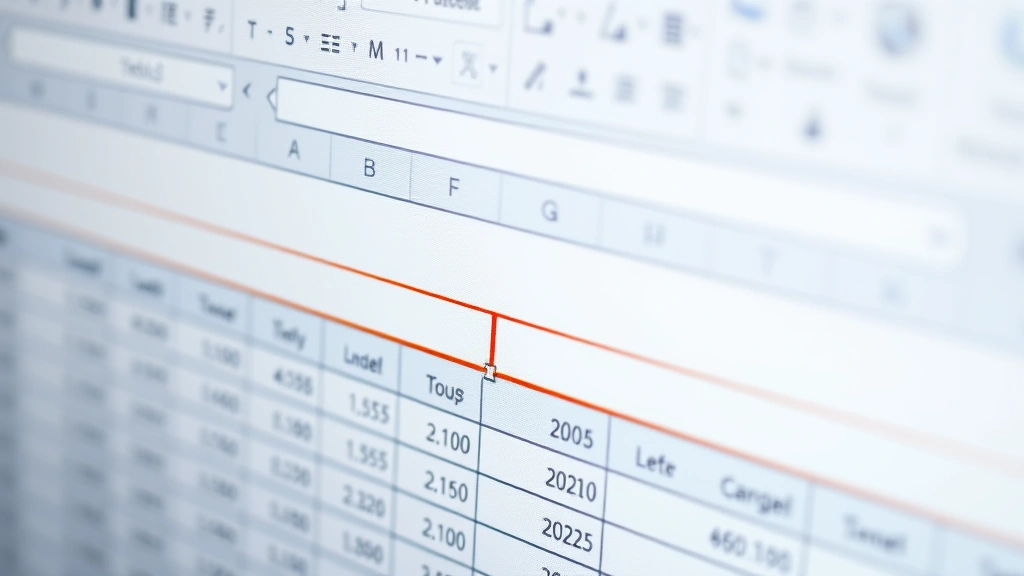
You’ll notice a slightly thicker line appearing below your frozen row. This visual indicator shows exactly where the freeze boundary is. Now scroll down—your header row stays put while the data below moves. That’s it. You’ve successfully locked the row.

Freezing Multiple Rows at Once
Sometimes one header row isn’t enough. Maybe you’ve got headers, subheaders, and a summary row at the top that all need to stay visible. No problem—you can freeze as many rows as you need.
The process is identical to freezing a single row, but you’ll click on the row below all the rows you want to freeze. So if you want to freeze Rows 1, 2, and 3, you’d click anywhere in Row 4 before opening the View menu and selecting Freeze Panes.
Excel will freeze everything above that line, giving you the flexibility to keep multiple reference rows visible. This is particularly useful for complex spreadsheets with multiple header levels or when you’re working with data that has summary rows interspersed throughout.
The key thing to remember: click the row below your freeze point. It’s the most common mistake people make, and it’s worth double-checking before you freeze.
Freezing Rows and Columns Together
Here’s where it gets really powerful. What if you’ve got row headers on the left side of your spreadsheet and column headers across the top? You can freeze both simultaneously.
The Setup
Let’s say your data starts in cell B2—Row 1 contains column headers, and Column A contains row labels. You want both to stay visible while scrolling.
The Steps
Click on cell B2 (the intersection point where your data actually begins). Then navigate to View → Freeze Panes. Excel will freeze Row 1 and Column A, keeping both your row and column headers visible as you navigate through the entire dataset.
This is where the magic happens. You can scroll right, and Column A stays. You can scroll down, and Row 1 stays. You can do both, and they both stay. It’s like having anchor points on two axes simultaneously, which dramatically improves your ability to understand large, complex datasets at a glance.

Unfreezing Rows: How to Undo the Lock
Changed your mind? Decided the freeze isn’t working for your workflow? Unfreezing is just as simple as freezing.
Go back to View → Freeze Panes, and you’ll notice the button now says Unfreeze Panes (or you’ll see the option in the dropdown). Click it once, and your freeze is removed. Everything goes back to normal scrolling behavior.
There’s no penalty for unfreezing—you’re not losing data or changing anything about your spreadsheet’s content. You’re simply toggling the visual behavior back to the default.
Advanced Locking Techniques
Beyond the basic freeze, Excel offers some additional options worth knowing about.
Freeze First Row
For the ultra-common case of wanting to lock only your top header row, Excel provides a shortcut. In the View menu, select Freeze Panes → Freeze First Row. This automatically freezes Row 1 without you having to select a position first. It’s convenient when you’re working with standard spreadsheet layouts.
Freeze First Column
Similarly, if you’ve got row labels in Column A that you want to keep visible while scrolling right, use Freeze Panes → Freeze First Column. This locks Column A in place.
Combining with Other Features
Freezing works beautifully with other Excel features. If you’re also interested in improving readability, you might want to explore how to wrap text in Excel to make your headers more compact. Or, if you’re building data entry forms, combining freezing with how to add a drop down list in Excel creates a professional, user-friendly interface.
For those who prefer alternative terminology or want a deeper dive into the mechanics, how to pin a row in Excel covers similar ground from a slightly different angle. And if you want to explore the broader freezing landscape, our guide on how to freeze a row in Excel offers comprehensive coverage of all scenarios.
Troubleshooting Common Issues
The Freeze Isn’t Working as Expected
Most often, this happens because you clicked on the wrong row. Remember: you need to click below the row you want to freeze. If your header row isn’t staying put, go back and select the correct position, then reapply the freeze.
I Can’t See the Freeze Line
The visual indicator (that slightly thicker line) might be subtle depending on your screen resolution and Excel theme. Try scrolling to confirm the freeze is actually working. If your header row stays while the data moves, the freeze is active even if you can’t see a prominent line.
Freezing Isn’t Available (Grayed Out)
This typically means you’re working with a protected sheet. Check if the sheet is password-protected. If it is, you’ll need the password to unprotect it before you can apply freezing.
I Froze Multiple Rows, But Only Some Stay Frozen
Double-check your selection point. You should have clicked on the row below all the rows you wanted to freeze. If only some are frozen, you likely clicked too high. Unfreeze and try again with the correct row selection.
Sharing Frozen Spreadsheets
Good news: when you share a spreadsheet with frozen panes, the freeze settings travel with the file. Your colleagues will see the same frozen rows you set up. However, they can unfreeze on their end if they prefer, and their changes won’t affect your original file’s settings.
Frequently Asked Questions
Can I freeze rows in Google Sheets?
Yes, Google Sheets has similar functionality. Click on the row below where you want to freeze, then go to View → Freeze and select the number of rows you want to freeze. The concept is identical, though the interface is slightly different.
Will freezing rows protect my data from being edited?
No. Freezing is purely visual—it keeps rows visible while scrolling but doesn’t prevent anyone from editing or deleting them. If you need actual protection, you’ll need to use Excel’s sheet protection features, which involve passwords and permissions.
How many rows can I freeze at once?
Technically, you can freeze quite a lot of rows, but practically speaking, you’re limited by your screen real estate. If you freeze too many rows, you won’t have much space left to view your actual data. Most use cases involve freezing one to three rows.
Can I freeze rows and columns in different sheets separately?
Absolutely. Each sheet in your workbook has its own freeze settings. You can freeze rows in Sheet1, freeze different rows in Sheet2, and leave Sheet3 completely unfrozen. The settings are independent for each sheet.
What’s the difference between freezing and splitting?
Splitting (also in the View menu) creates movable dividers that let you scroll independently in different areas. Freezing locks rows and columns in place. Splitting offers more flexibility but is less commonly used for standard spreadsheet work.
Does freezing affect printing?
No. Frozen panes are a screen display feature only. When you print your spreadsheet, everything prints normally without any indication of where the freeze was set. The frozen rows will appear on every page if they’re included in your print range, but that’s a separate print setting.
Can I freeze non-contiguous rows?
No. Freezing always works from the top down. You can only freeze complete rows starting from Row 1. You can’t freeze Row 1 and Row 3 while leaving Row 2 unfrozen, for example.


