Create Drop-Down List in Excel: Easy Steps for Better Data Management

Drop-down lists in Excel are one of the most powerful yet underutilized features for organizing and managing data efficiently. Whether you’re building a budget spreadsheet, creating an inventory tracker, or designing a survey form, drop-down lists ensure consistent data entry and reduce errors dramatically. This guide walks you through everything you need to know about how to make drop down list in excel, from basic setup to advanced customization techniques.

Data validation through drop-down lists keeps your spreadsheets clean and professional. Instead of allowing free-text entries that might contain typos or inconsistencies, drop-down lists restrict options to predefined choices. This is particularly valuable in collaborative environments where multiple team members contribute data. By implementing drop-down lists, you create a standardized system that everyone can follow, making your spreadsheet more reliable and easier to analyze.

What Are Drop-Down Lists and Why Use Them

A drop-down list in Excel is a cell containing a small arrow that users can click to reveal a list of predefined options. These lists are created using Excel’s Data Validation feature, which restricts cell entries to specific values you define. When someone clicks on a cell with a drop-down list, they see all available options and can select one instead of typing manually.

The benefits of drop-down lists extend far beyond simple organization. Data consistency is perhaps the most obvious advantage—when all entries come from the same list, you eliminate spelling variations and typos. This matters enormously when you’re later sorting, filtering, or analyzing data. A column containing “Yes,” “yes,” and “YES” creates three different categories in most analysis tools, but a drop-down list ensures uniform capitalization.

Drop-down lists also improve user experience by making data entry faster. Instead of typing complete entries, users simply click and select. This is especially valuable for long entries or when working with mobile devices. Additionally, drop-down lists serve as data documentation—they show users what options are acceptable, reducing confusion and support requests.

For team collaboration, drop-down lists establish quality control. When designing spreadsheets for others to use, you’re essentially creating guardrails that guide people toward correct data entry. This is why many professional templates and FixWiseHub Blog recommendations emphasize data validation as a best practice.

Basic Method: Creating Drop-Down Lists with Data Validation

The fundamental approach to creating drop-down lists involves Excel’s Data Validation tool. This method works identically in Excel for Windows, Excel for Mac, and Excel Online. Here’s the step-by-step process:

Step 1: Select Your Target Cell or Range

First, click on the cell where you want the drop-down list to appear. If you need the same drop-down in multiple cells, select the entire range at once. You can select a range by clicking the first cell, holding Shift, and clicking the last cell. Alternatively, click a cell and drag to select multiple adjacent cells. For non-adjacent cells, hold Ctrl (or Cmd on Mac) while clicking individual cells.

Step 2: Access Data Validation

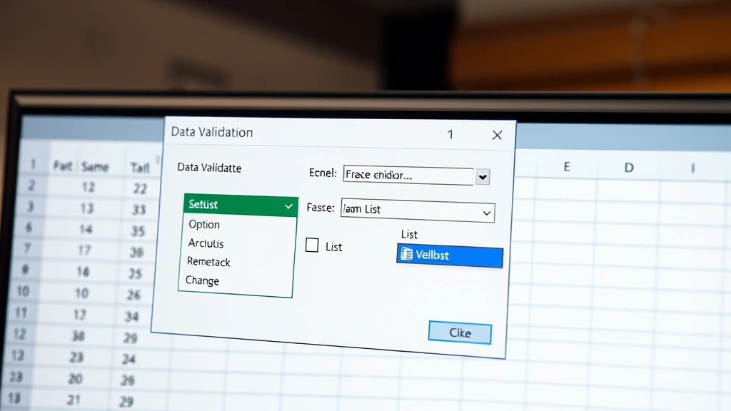
Navigate to the Data menu in Excel’s ribbon. Look for the “Data Validation” option—it’s typically in the Data Tools section. Click on it to open the Data Validation dialog box. In Excel Online, this option appears under the Data menu as well. The dialog contains several tabs: Settings, Input Message, and Error Alert.

Step 3: Configure Validation Settings

In the Settings tab, locate the “Allow” dropdown menu. Change it from “All” to “List.” This tells Excel that you want to restrict entries to specific values. Once you select “List,” a new field appears labeled “Source” where you’ll enter your options.

Step 4: Enter Your List Items

In the Source field, type your drop-down options separated by commas. For example, if you’re creating a status list, you might enter: Pending,In Progress,Completed,On Hold. Excel automatically recognizes the commas as separators and creates individual list items. Keep entries concise—ideally under 50 characters each—so they display properly in the cell.

Step 5: Configure Error Handling (Optional)

Click the “Error Alert” tab to set up a message that appears if someone tries to enter a value not on your list. Choose an alert style: “Stop” prevents invalid entries entirely, “Warning” allows them but displays a caution, and “Information” provides a message without restricting entry. Add a title and message explaining what values are acceptable.

Step 6: Add Input Message (Optional)

The “Input Message” tab lets you display helpful text when someone clicks the cell. This might say “Select a status from the list” or “Choose a department name.” Input messages improve user experience by clearly explaining what the cell expects.

Step 7: Apply and Test

Click OK to apply the data validation. Click on your cell—you should see a small dropdown arrow appear. Click the arrow to verify your list displays correctly. Select an item to confirm the selection works.

Using Cell Range as Drop-Down Source

Rather than typing list items directly into the Source field, you can reference a range of cells containing your options. This approach offers significant advantages for managing large lists or lists that change frequently.

Creating a Source List

First, create a separate area in your spreadsheet containing your drop-down options. Many users designate a specific column, perhaps on a different sheet, for maintaining these lists. For example, you might create a “Lists” sheet and put all your status options in column A (rows 1-5). This centralized approach makes updating options easy—change the source list once, and all drop-downs automatically reflect the update.

Referencing the Range

When setting up data validation, instead of typing items in the Source field, reference your list range. Use the format =SheetName!A1:A5 or simply =A1:A5 if the list is on the same sheet. Excel recognizes this as a range reference and pulls values from those cells. If your list is on a different sheet named “Lists,” you’d enter =Lists!A1:A5.

Dynamic Lists with INDIRECT Function

For advanced users, the INDIRECT function enables dynamic list sizing. Instead of specifying exact cell ranges, you can create a formula that automatically adjusts to include all non-empty cells in a column. This is particularly useful when your list grows over time. The formula might look like =INDIRECT(“Lists!A1:A”&COUNTA(Lists!A:A)), which counts non-empty cells and adjusts the range accordingly.

Advantages of Range-Based Lists

Range-based drop-down sources offer several benefits. Maintenance becomes simpler—you edit the source list in one location, and all connected drop-downs update automatically. Collaboration improves because team members can see available options by checking the source list. Scalability increases because adding new options doesn’t require editing data validation settings. This approach aligns with professional spreadsheet design principles emphasized by resources like Family Handyman for general project management.

Advanced Techniques: Dependent Drop-Down Lists

Dependent (or cascading) drop-down lists create a hierarchy where the options in one drop-down depend on the selection in another. This advanced technique is invaluable for complex data scenarios. For instance, if you have a “Country” drop-down and a “City” drop-down, selecting “United States” might limit city options to US cities only.

Setting Up Source Lists

Begin by organizing your data hierarchically. Create separate named ranges for each category. If building a regional sales tracker, you might have ranges named “North_Region,” “South_Region,” “East_Region,” and “West_Region,” each containing relevant cities or territories. Use Excel’s Name Manager (accessible via Formulas menu) to create these named ranges efficiently.

Creating the Primary Drop-Down

Set up your first drop-down normally, using a list of categories (regions, countries, departments). This is your primary selector that controls subsequent lists.

Building the Dependent Drop-Down

For the dependent drop-down, use the INDIRECT function in the Source field. If your primary drop-down is in cell A1 and contains region names, your dependent drop-down source would be =INDIRECT(A1). This tells Excel to use whatever value appears in A1 as the name of a range to pull from. When someone selects “North_Region” in A1, the dependent drop-down automatically displays options from the North_Region named range.

Extending to Multiple Levels

You can create three or more levels of dependent lists by chaining the INDIRECT function. A third-level drop-down might reference the second-level selection, creating a country-region-city hierarchy. This approach scales to any depth your data structure requires.

Formatting and Customizing Your Drop-Down Lists

Beyond basic creation, Excel offers several customization options to make your drop-down lists more user-friendly and visually integrated with your spreadsheet design.

Adding Helpful Messages

Use the Input Message tab in Data Validation to display instructions when users select a cell. A message like “Select the project status” provides context. Keep messages concise—Excel displays them in small tooltip-style boxes. The Input Title appears in bold above the message, so use it for brief labels like “Status Selection.”

Styling Drop-Down Cells

Format cells containing drop-downs distinctly so users recognize them as interactive. Apply a light background color (light blue or light gray works well) to make drop-down cells visually distinct from regular cells. Add borders to emphasize the cells’ importance. These visual cues help users understand where they can make selections.

Restricting List Length

Excel displays drop-down lists in a scrollable box. If your list exceeds 20-30 items, consider whether users really need all options visible at once. Long lists become cumbersome to navigate. Instead, consider creating dependent drop-downs that filter options into smaller, more manageable groups. This improves usability significantly.

Allowing Blank Entries

By default, data validation requires selections from your list. If some cells should remain empty, check the “Ignore blank” option in the Settings tab. This allows users to leave cells empty without triggering error messages, which is often necessary for optional fields.

Case Sensitivity

Data validation is not case-sensitive by default—”Yes” and “yes” are treated identically. This is usually desirable for consistency, but if your data structure requires case-sensitive matching, you can achieve this using formulas instead of simple lists.

Troubleshooting Common Drop-Down Issues

Even experienced Excel users encounter problems with drop-down lists. Understanding common issues and their solutions saves considerable frustration.

Drop-Down Arrow Not Appearing

If you’ve created data validation but don’t see the dropdown arrow, check that your cell is selected. The arrow only appears when the cell is active. If the arrow still doesn’t appear, verify that data validation was actually applied—go to Data Validation and confirm your settings are still there. Sometimes Excel loses validation settings if cells are deleted or moved.

INDIRECT Function Not Working

When using INDIRECT with named ranges, ensure your named range names exactly match what you’re referencing in the formula. Excel is unforgiving about typos in range names. Also verify that named ranges are defined at the workbook level (not sheet level) unless you specifically want sheet-level scope. Use the Name Manager to double-check range definitions.

List Items Appearing Truncated

If your drop-down list items are cut off in the display, your entries might be too long. Excel limits the visible width of drop-down lists. Shorten entries or use abbreviations. Alternatively, use the Input Message feature to display full text as a tooltip when users hover over the cell.

Validation Not Preventing Invalid Entries

If users can enter values not on your list despite having data validation, check your Error Alert settings. An “Information” alert style allows invalid entries—change it to “Stop” to prevent them. Also verify that “Show error alert when invalid data is entered” is checked.

Drop-Down Breaking After Copying

When you copy cells with drop-downs, the validation typically copies with them, which is good. However, if you’re using INDIRECT with relative references and copy cells, the references might shift incorrectly. Use absolute references (with dollar signs like $A$1) when creating dependent lists to ensure references don’t change when copied.

Performance Issues with Large Lists

If your drop-down contains thousands of items, performance might suffer. Consider splitting large lists into categories using dependent drop-downs. Alternatively, use data entry forms or filtered lists rather than massive drop-down menus. This Old House approach to systematic organization applies here—breaking complex problems into manageable pieces improves overall functionality.

FAQ

Can I use drop-down lists in Excel Online?

Yes, Excel Online supports data validation and drop-down lists with the same basic functionality as desktop Excel. Access it through the Data menu. Some advanced features like dependent lists using INDIRECT work identically in online versions.

How do I delete a drop-down list?

Select the cell or range containing the drop-down, go to Data Validation, and click “Clear All.” This removes all validation rules from the selected cells. The cells return to normal text entry mode.

Can I copy drop-down lists to other cells?

Absolutely. Select a cell with a drop-down, copy it (Ctrl+C), then select your target range and paste (Ctrl+V). The validation rules copy along with the cell formatting. This is much faster than creating each drop-down individually.

What’s the maximum number of items in a drop-down list?

Excel doesn’t have a strict limit, but practical usability declines with very large lists. Most experts recommend keeping lists under 100 items. For larger datasets, use dependent drop-downs or consider alternative approaches like filtered lists.

Can I sort drop-down list items alphabetically?

If your source list is in cells, simply sort those cells alphabetically. When you use range references, the drop-down automatically reflects the source list’s order. For comma-separated lists entered directly in validation, you’ll need to manually arrange them alphabetically.

How do I make a drop-down list case-insensitive?

Drop-down lists are case-insensitive by default. If you need case-sensitive validation, you’ll need to use custom formulas in data validation rather than simple list validation.

Can I use formulas in drop-down lists?

You can reference cells containing formulas as your validation source, but you cannot enter formulas directly as list items. Create a helper column with formulas that generate your list values, then reference that column in your data validation.