Freeze Columns in Excel: Expert Tips & Tricks

Working with large spreadsheets can be overwhelming, especially when you’re scrolling horizontally through dozens of columns while trying to keep track of row headers. This is where Excel’s freeze columns feature becomes invaluable. By freezing specific columns, you create a locked reference point that remains visible while you navigate through the rest of your data. Whether you’re managing financial reports, inventory lists, or project timelines, mastering this feature will significantly improve your productivity and reduce errors.

Freezing columns in Excel is one of those simple yet powerful features that many users overlook. When properly implemented, it transforms how you interact with large datasets, allowing you to maintain context while exploring data. This comprehensive guide will walk you through every method available, from basic freezing techniques to advanced configurations that professional analysts use daily.

Understanding Excel Freeze Panes Basics

Before diving into the technical steps, it’s important to understand what freezing columns actually does. When you freeze columns in Excel, you’re essentially splitting your worksheet into separate panes. The frozen columns remain stationary on your screen while the unfrozen columns scroll freely. This is particularly useful when your spreadsheet contains identifier columns on the left—like employee names, product IDs, or dates—that you want visible at all times.

The freeze feature works by creating a visual division in your worksheet. Excel recognizes this division and prevents the frozen area from moving when you scroll. Unlike simply hiding columns, which removes them from view entirely, freezing keeps them visible and accessible. This distinction is crucial for maintaining data integrity and workflow efficiency. When you’re working with spreadsheets containing hundreds of rows and columns, this feature becomes absolutely essential.

Understanding the mechanics helps you use the feature more effectively. The freeze panes function operates on a grid system—you select a cell, and everything to the left and above that cell becomes frozen. This means your selection point is critical. Choosing the wrong cell can result in freezing too many or too few columns, requiring you to undo and restart.

How to Freeze a Single Column

Freezing a single column is the most common use case and the easiest to execute. Most spreadsheets benefit from keeping the first column frozen, as it typically contains important identifiers. Here’s the step-by-step process:

1. Open your Excel spreadsheet and locate the column you want to freeze. In most cases, this will be column A.
2. Click on the column header to the right of the column you wish to freeze. For example, if you want to freeze column A, click on column B’s header.
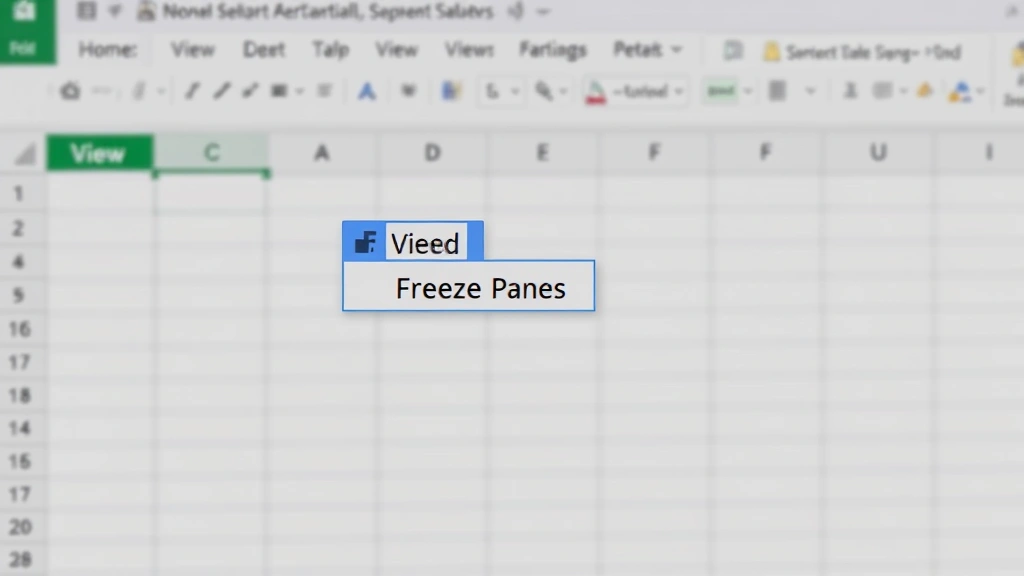
3. Navigate to the View tab in the Excel ribbon at the top of your screen.
4. Look for the Freeze Panes option. Click on it to reveal a dropdown menu with several options.
5. Select Freeze Panes from the dropdown. This will immediately freeze all columns to the left of your selection.
6. You’ll notice a thin line appears to the right of the frozen column, indicating the freeze boundary.

Once you’ve frozen a single column, scroll horizontally through your spreadsheet to verify the freeze is working correctly. The frozen column should remain visible on the left side of your screen while the other columns move freely. This visual confirmation ensures your data remains properly contextualized as you navigate.

Freezing Multiple Columns Simultaneously

Many professional spreadsheets require freezing more than one column. For instance, a sales database might need both an employee ID column and a department column frozen to provide complete context. The process is nearly identical to freezing a single column, with one key difference: your cell selection determines how many columns get frozen.

To freeze multiple columns, follow these steps:

1. Identify which columns you need to freeze. Count them carefully—this number determines your selection strategy.
2. Click on the column header that immediately follows your last frozen column. If you want to freeze columns A, B, and C, you’ll click on column D.
3. Access the View tab and select Freeze Panes from the dropdown menu.
4. All columns to the left of your selected column are now frozen.
5. Test your freeze by scrolling right to ensure all intended columns remain visible.

This method works because Excel freezes everything to the left of your cursor position. By selecting the column immediately after your desired frozen range, you ensure the correct columns remain locked. This approach scales effectively whether you’re freezing two columns or ten.

When working with complex spreadsheets from data management guides, you’ll often need to adjust your frozen columns as your data structure evolves. Having this skill mastered allows you to adapt quickly to changing requirements.

Freeze Columns and Rows Together

Professional data analysts frequently need to freeze both columns and rows simultaneously. Imagine a financial spreadsheet with months across the top and expense categories down the left side. You’d want both the category column and the month row frozen for easy reference. Excel handles this elegantly through a single selection.

Here’s how to freeze both columns and rows:

1. Locate the cell that sits at the intersection of your desired freeze boundaries. If you want to freeze column A and row 1, select cell B2.
2. Navigate to the View tab and click Freeze Panes.
3. Both the column to the left and the row above your selected cell are now frozen.
4. Scroll both horizontally and vertically to confirm both dimensions are locked properly.

This technique is powerful for complex datasets. The frozen areas create a stable reference frame that helps prevent data entry errors and makes analysis more efficient. When you’re comparing values across different sections of a large spreadsheet, having both contextual markers frozen dramatically improves accuracy.

For spreadsheets with multiple frozen dimensions, consider using our comprehensive how-to guides to explore other organizational strategies that complement freezing techniques.

Advanced Freezing Techniques

Beyond basic freezing, Excel offers several advanced configurations for power users. The Freeze Panes dropdown menu contains options beyond the standard freeze:

Freeze First Column: This option automatically freezes column A without requiring cell selection. It’s a quick shortcut when you know you only need the first column locked. Simply access View → Freeze Panes → Freeze First Column.

Freeze Top Row: Similarly, this freezes your header row (typically row 1) without additional configuration. Use this when you have column headers that need to remain visible while scrolling down through data.

Custom Freeze Configurations: For non-standard layouts, the general Freeze Panes option provides maximum flexibility. You can freeze any combination of columns and rows by selecting the appropriate cell before activating the freeze.

Advanced users often combine freezing with other Excel features for enhanced functionality. For example, you might freeze columns while also using our dedicated Excel column freezing guide to explore filter options that work seamlessly with frozen panes. Filters applied to frozen columns remain accessible, allowing you to sort and filter data while maintaining your frozen reference columns.

Another advanced technique involves using frozen panes with conditional formatting. When you apply color-coding or highlighting to cells in a frozen column, it remains visible and effective across the entire scrollable area, providing visual organization throughout your dataset.

Unfreezing and Adjusting Your Setup

Freezing isn’t permanent. Excel makes it easy to unfreeze columns when your needs change or when you want to reconfigure your frozen panes. The unfreezing process is straightforward:

1. Navigate to the View tab in the ribbon.
2. Click on Freeze Panes to open the dropdown menu.
3. Select Unfreeze Panes from the options.
4. All previously frozen columns and rows are now unlocked and will scroll normally.

If you need to adjust which columns are frozen rather than removing the freeze entirely, you must unfreeze first, then select a new freeze point and reactivate the feature. There’s no direct “re-freeze” option, so this two-step process is necessary for configuration changes.

When adjusting your freeze setup, consider saving your file before making changes. This allows you to quickly revert if the new configuration doesn’t work as intended. Many users maintain multiple versions of complex spreadsheets with different freeze configurations for different analysis tasks.

Common Mistakes and Solutions

Mistake 1: Freezing the Wrong Columns

The most common error occurs when users select the wrong column header before freezing. Remember: Excel freezes everything to the left of your selection. If you want to freeze column A, select column B. Double-check your selection before confirming the freeze.

Mistake 2: Forgetting About Frozen Panes When Copying Data

When copying data from a frozen spreadsheet, the freeze boundaries don’t copy to the new location. If you paste frozen data into a new spreadsheet without reapplying the freeze, your new spreadsheet won’t have the same configuration. Remember to reapply freezing in your destination spreadsheet.

Mistake 3: Confusing Freeze Panes with Column Hiding

Some users hide columns thinking it’s the same as freezing. Hidden columns are removed from view entirely and aren’t accessible without unhiding them. Frozen columns remain visible and functional. These are distinctly different features serving different purposes.

Mistake 4: Applying Freeze to the Wrong Row/Column Combination

When freezing both rows and columns, selecting the wrong cell creates misaligned freezes. Always count carefully: if you want to freeze three columns and two rows, select cell D3 before freezing. The row number and column letter of your selection determine the freeze boundaries.

Solution Strategy: If you make a mistake, simply unfreeze and restart. There’s no penalty for undoing and reconfiguring your freeze setup. Taking an extra moment to verify your selection prevents frustration later.

Freezing Columns in Different Excel Versions

Excel has evolved significantly over the years, and the freeze panes feature remains consistent across modern versions. However, older versions had slightly different interfaces:

Excel 2016 and Later (Windows and Mac): The current standard interface applies. Access Freeze Panes through the View tab. The process described throughout this guide applies directly to these versions.

Excel 2013 and 2010: These versions use the same View tab interface, though the ribbon layout may differ slightly. The Freeze Panes option is still located in the View tab, and the functionality is identical.

Excel Online (Web Version): Excel Online supports freezing through the View menu. The process is similar, though some advanced options may be limited compared to desktop versions. Access Freeze Panes through the View tab, then select your freeze configuration.

Excel for Mac: Mac users access the same Freeze Panes feature through the View menu in the ribbon. The functionality is identical to Windows versions, though menu locations may appear slightly different due to Mac interface conventions.

Regardless of your Excel version, the fundamental principle remains: select your freeze point, then activate Freeze Panes. This consistency makes the feature accessible to users across different platforms and versions.

For detailed information about Excel functionality across platforms, consult Microsoft’s official Office support documentation. For home office setup guidance that includes spreadsheet management, This Old House offers comprehensive home office organization tips.

FAQ

Can I freeze columns and rows at the same time in Excel?

Yes, absolutely. Select the cell at the intersection of your desired freeze boundaries. For example, to freeze column A and row 1, select cell B2, then activate Freeze Panes. Both dimensions will freeze simultaneously.

What’s the difference between freezing columns and hiding columns?

Freezing columns keeps them visible and accessible while you scroll through other data. Hiding columns removes them from view entirely. Frozen columns remain functional and visible; hidden columns must be unhidden to access them again.

How do I unfreeze columns in Excel?

Navigate to the View tab and click Freeze Panes, then select Unfreeze Panes. All previously frozen columns and rows will return to normal scrolling behavior.

Can I freeze non-adjacent columns?

No, Excel only allows freezing contiguous columns from the left edge of your spreadsheet. You can freeze columns A and B, but not columns A and C while leaving B unfrozen. To achieve non-adjacent freezing effects, consider hiding unwanted columns or reorganizing your data structure.

Does freezing affect printing?

Frozen panes don’t affect how your spreadsheet prints. When you print a frozen spreadsheet, all columns and rows print normally without freeze boundaries. The freeze is a viewing feature only and doesn’t impact printed output.

Will frozen columns remain frozen if I share the file?

Yes, freeze settings are saved with your Excel file. When you share a spreadsheet with frozen columns, other users will see the same freeze configuration when they open the file. This ensures consistent viewing across your team.

Can I freeze columns in a protected spreadsheet?

Freezing and protection are separate features. You can freeze columns in a protected spreadsheet, and the freeze will remain active. However, if sheet protection is enabled, users may not be able to modify the freeze settings, depending on protection parameters.

What if Freeze Panes option is grayed out?

If Freeze Panes appears grayed out, you may be in a view mode that doesn’t support freezing, such as Page Break Preview. Switch to Normal view through the View tab, and Freeze Panes should become available.