Strikethrough in Excel: Easy Steps for Beginners

Strikethrough formatting in Excel is a simple yet powerful tool that helps you mark items as completed, removed, or no longer relevant without deleting them. Whether you’re managing a to-do list, tracking inventory changes, or reviewing document edits, knowing how to apply strikethrough can save you time and keep your spreadsheets organized. This formatting option is available in all versions of Excel and takes just a few clicks to master.

Many beginners overlook this feature, but once you understand how to use it, you’ll find countless applications in your daily spreadsheet work. From project management to data organization, strikethrough helps maintain a clear visual record of changes while preserving original information. Let’s explore the different methods to apply strikethrough formatting and discover how it can improve your Excel workflow.

What is Strikethrough Formatting

Strikethrough formatting is a text effect that places a horizontal line through the middle of your text. In Excel, this feature allows you to visually indicate that content is outdated, completed, or removed without actually deleting the data. This is particularly useful when you need to maintain an audit trail or keep historical records visible alongside current information.

The strikethrough effect works on individual cells, entire rows, or specific text within cells. Unlike deleting content, strikethrough preserves the original information while clearly marking it as inactive or obsolete. This approach is especially valuable in collaborative spreadsheets where multiple people need to understand what changes have been made and why. You can combine strikethrough with other formatting options like color changes or font adjustments for even greater clarity.

Understanding when and how to use strikethrough properly will make your spreadsheets more professional and easier to read. It’s a formatting choice that shows attention to detail and helps prevent confusion when reviewing data. Many Excel users find that incorporating strikethrough into their workflow significantly improves document clarity and reduces miscommunication.

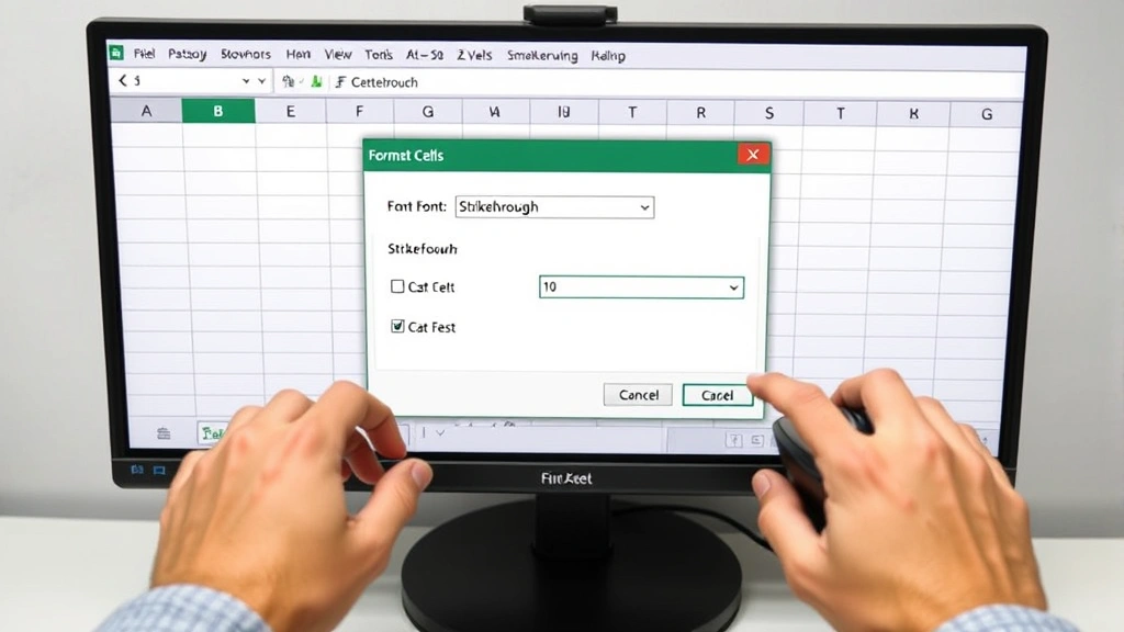
Method 1: Using the Format Cells Dialog

The Format Cells dialog is the most comprehensive way to apply strikethrough formatting in Excel. This method gives you access to all text formatting options in one convenient location. Here’s how to use it:

1. Select the cell or cells you want to format. Click on a single cell, or drag across multiple cells to select a range. You can also click the cell reference box and type a range like A1:A10.
2. Right-click on your selection to open the context menu. This menu appears at your cursor location and contains formatting options specific to your selection.
3. Choose “Format Cells” from the dropdown menu. This opens the Format Cells dialog box with multiple tabs for different formatting options.
4. Click the “Font” tab at the top of the dialog box. This tab contains all text formatting options including font, size, color, and effects.
5. Look for the “Effects” section in the Font tab. You’ll see a checkbox next to “Strikethrough.” Click this checkbox to enable the effect.
6. Click “OK” to apply the formatting. Your selected cells will now display strikethrough text.

This method is ideal when you want to apply strikethrough along with other formatting changes. For example, you might want to apply strikethrough and change the text color to gray simultaneously to make completed items stand out clearly. The Format Cells dialog allows you to make all these changes before clicking OK, which is more efficient than applying formatting in multiple steps.

Method 2: Using the Keyboard Shortcut

If you frequently use strikethrough formatting, the keyboard shortcut method is the fastest option. Excel provides a built-in shortcut that works on Windows and Mac systems, though the key combinations differ slightly.

For Windows users: Press Alt + H to open the Home tab ribbon, then press 4 to apply strikethrough. Alternatively, some Excel versions support Alt + Shift + 5 as a direct strikethrough shortcut, though this may vary depending on your Excel version and keyboard layout.

For Mac users: Press Command + Shift + X to toggle strikethrough on and off. This shortcut works consistently across different Mac Excel versions and is easy to remember once you’ve used it a few times.

To use the keyboard shortcut method, first select the cell or text you want to format, then press the appropriate shortcut for your system. The strikethrough formatting will apply immediately without opening any dialog boxes. This method is perfect when you’re working quickly and want to maintain your workflow without interruption. You can press the same shortcut again to remove strikethrough formatting from the same selection.

Method 3: Using the Ribbon Menu

The Ribbon menu provides a visual way to apply strikethrough formatting. This method is helpful if you prefer seeing formatting options displayed on your screen rather than memorizing keyboard shortcuts.

1. Select your cell or range of cells that you want to format with strikethrough.
2. Look at the Home tab in the Ribbon at the top of your Excel window. The Home tab contains most common formatting options.
3. Find the Font group in the Ribbon. This section contains font name, size, and color options.
4. Click the small arrow button next to the font formatting options. This opens the Font dialog box, which is similar to the Format Cells dialog accessed through right-clicking.
5. Navigate to the Font tab and check the Strikethrough checkbox in the Effects section.
6. Click OK to apply the formatting.

Some newer versions of Excel include a strikethrough button directly in the Ribbon. If your version has this feature, you can simply click the strikethrough button icon without opening any dialog boxes. Check the Font group in your Home tab to see if this quick-access button is available. If it’s not visible, you can customize your Ribbon to add it for faster access.

Removing Strikethrough Text

Removing strikethrough formatting is just as easy as applying it. You might need to remove strikethrough if you made a mistake, changed your mind, or want to reactivate previously marked items. The process varies slightly depending on which method you used to apply the formatting.

Using Format Cells: Select the strikethrough text, right-click, choose Format Cells, click the Font tab, uncheck the Strikethrough checkbox, and click OK. This method works regardless of how the strikethrough was originally applied.

Using the Keyboard Shortcut: Simply select the strikethrough text and press the same keyboard shortcut you used to apply it. The shortcut toggles strikethrough on and off, so pressing it again removes the formatting instantly. This is the fastest method if you’re already comfortable with keyboard shortcuts.

Using the Ribbon: Select your strikethrough text, open the Font dialog through the Ribbon, uncheck Strikethrough, and click OK. You can also use the quick-access strikethrough button if your version of Excel has one visible in the Ribbon.

If you want to remove strikethrough from multiple cells at once, select all the cells containing strikethrough text before using any of these methods. Excel will remove the formatting from all selected cells simultaneously, saving you time when working with large datasets.

Advanced Strikethrough Techniques

Once you’ve mastered basic strikethrough formatting, you can explore more advanced techniques to enhance your spreadsheet management. These methods can help you create more sophisticated and professional-looking documents that communicate information more effectively.

Combining Strikethrough with Conditional Formatting: You can use Excel’s conditional formatting feature alongside strikethrough to automatically apply strikethrough to cells that meet specific criteria. For example, you might want to automatically strikethrough all items with a due date in the past or all inventory items with zero quantity. This automation reduces manual formatting work and ensures consistency across your spreadsheet. To set this up, access the Conditional Formatting menu in the Home tab, create a new rule, and specify both the condition and the strikethrough formatting to apply.

Creating Visual Status Indicators: Combine strikethrough with color formatting to create a clear visual system. For instance, you might use red text with strikethrough for deleted items, gray text with strikethrough for completed tasks, and normal formatting for active items. This multi-layered approach makes it immediately clear at a glance which items are current and which are historical. Document your color and formatting system in a legend at the top of your spreadsheet so collaborators understand your conventions.

Using Strikethrough in Formulas: While you can’t directly apply strikethrough through formulas, you can use formulas to identify which cells should receive strikethrough formatting. For example, create a formula that checks if a task completion date is filled in, then manually apply strikethrough to those rows. Alternatively, use the FixWise Hub Blog resources to learn about creating more sophisticated spreadsheet systems that track status changes automatically.

Protecting Strikethrough Formatting: If you’re sharing your spreadsheet with others, consider protecting cells to prevent accidental removal of strikethrough formatting. You can set up sheet protection that allows users to enter data in certain cells while preventing them from modifying formatting. This ensures that your visual status system remains intact even when others are editing the spreadsheet.

Common Uses for Strikethrough

Understanding practical applications for strikethrough formatting will help you implement it effectively in your daily work. Many professionals use strikethrough in ways that significantly improve their productivity and organization.

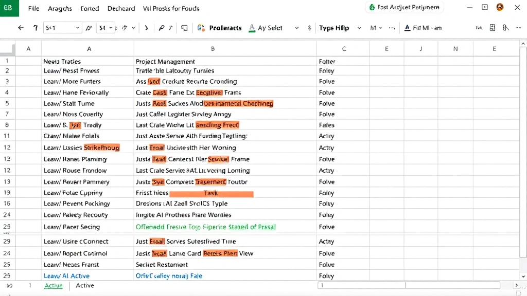
Project Management and Task Tracking: Use strikethrough to mark completed tasks in your project plan. When a task is finished, apply strikethrough instead of deleting the row. This creates a visible record of completed work and helps team members understand what’s been accomplished. Project managers often find that this approach is more informative than simply removing completed tasks, as it shows the project’s progress over time.

Inventory Management: When items are removed from inventory or discontinued, strikethrough the entries instead of deleting them. This preserves your historical inventory data while clearly indicating which items are no longer available. This approach is especially useful when you need to maintain records for auditing or accounting purposes.

Budget and Financial Tracking: Apply strikethrough to budget line items that have been removed or revised. This helps finance teams track budget changes while maintaining a clear audit trail. Instead of replacing old budget figures with new ones, you can keep both visible with strikethrough indicating the outdated version.

Content Review and Editing: When reviewing documents collaboratively, strikethrough indicates text that should be removed without actually deleting it. This gives other reviewers a chance to see what changes have been suggested and potentially restore content if needed. It’s a non-destructive editing approach that works well in collaborative environments.

Data Quality Indicators: Mark data that you suspect is inaccurate or needs verification with strikethrough. This signals to other users that the information may be unreliable without removing it from the spreadsheet. Once you’ve verified the data, you can remove the strikethrough formatting to indicate that it’s been confirmed as accurate.

Meal Planning and Grocery Lists: Similar to how you might store green onions after using them, strikethrough items on your grocery list as you purchase them. This approach keeps your shopping list intact while showing which items you’ve already obtained. You can reuse the same list for future shopping trips by removing strikethrough from all items.

Recipe Organization: When testing recipes or planning meals, use strikethrough to mark recipes you’ve already tried or ingredients you’ve already used. This is particularly helpful if you’re making a latte at home and tracking different variations or if you’re cleaning a coffee maker and tracking maintenance tasks.

FAQ

Can I apply strikethrough to only part of the text in a cell?

Yes, you can apply strikethrough to partial cell content. Double-click the cell to enter edit mode, then select only the text you want to format. Use the Format Cells dialog or keyboard shortcut to apply strikethrough to just that selected text. This is useful when you want to mark part of a cell’s content as outdated while keeping the rest active.

Does strikethrough formatting work in Excel Online?

Strikethrough formatting is supported in Excel Online, though the interface differs slightly from desktop Excel. You can access it through the Home tab in the Ribbon or by using keyboard shortcuts. Excel Online provides the same formatting functionality as desktop versions for most common features including strikethrough.

Can I search for cells with strikethrough formatting?

Excel’s Find & Replace feature allows you to search for cells with specific formatting, including strikethrough. Open Find & Replace (Ctrl+H), click Format options, and specify strikethrough as a search criterion. This is helpful when you need to find all strikethrough cells in a large spreadsheet or remove strikethrough formatting from multiple cells at once.

Will strikethrough formatting print correctly?

Yes, strikethrough formatting prints exactly as it appears on your screen. When you print your spreadsheet, all strikethrough text will show the horizontal line through the middle. Make sure your printer settings are configured to print formatting, which is typically the default setting.

Can I use strikethrough in Excel charts or pivot tables?

Strikethrough formatting can be applied to data in cells, but it doesn’t automatically appear in charts based on that data. Charts display the actual values rather than the cell formatting. For pivot tables, strikethrough formatting may not persist when the pivot table refreshes, so it’s best to use other formatting methods for frequently updated pivot tables.

How do I apply strikethrough to an entire row?

Click the row number on the left side of the spreadsheet to select the entire row. Then use any of the three methods described in this guide to apply strikethrough. All cells in that row will receive strikethrough formatting. Be cautious with this approach if your row contains headers or other important information you don’t want to mark as obsolete.

Is there a way to automatically apply strikethrough based on dates?

Yes, you can use conditional formatting to automatically apply strikethrough to cells based on date criteria. Set up a conditional formatting rule that checks if a date is in the past or meets other criteria, then apply strikethrough as the formatting effect. This automation is particularly useful for task lists where you want to automatically mark overdue items.

Can multiple users see strikethrough formatting in shared Excel files?

Yes, strikethrough formatting is preserved in shared Excel files and cloud-based spreadsheets like OneDrive or SharePoint. All users who access the file will see the strikethrough formatting applied by other users. This makes strikethrough an effective communication tool in collaborative environments where teams need to track changes and status updates.